Tutorials (MATLAB)

This tutorial walks you through how to use the DANT package to track neurons across sessions. It is designed to help you prepare your data and run the code effectively. Before starting, make sure DANT is installed correctly. If you have not installed it yet, please refer to the Installation section.

Prepare the data

An example dataset is available here. You can download it and follow the steps below to run the full example. You can also use your own dataset by following the same workflow.

To use DANT, prepare your data in a specific format. The data should be a 1 x n struct array named spikeInfo with the following fields:

Field name	Type	Explanation
`SessionIndex`	1 x 1 int	indicates the session. It should start from 1 and be continuous without any gaps.
`SpikeTimes`	1 x n double	spike times in milliseconds
`Waveform`	n_channel x n_sample double	mean waveform in uV
`Xcoords`	n_channel x 1 double	x coordinates of each channel
`Ycoords`	n_channel x 1 double	y coordinates (depth) of each channel
`Kcoords`	n_channel x 1 double	shank index of each channel (for multi-shank probes)
`PETH`	1 x n double	peri-event time histogram (optional)

Crucially, the waveforms used in this analysis must not be whitened, unlike those processed by Kilosort. Avoid direct use of waveforms from temp_wh.dat and refrain from using whitening_mat_inv.npy or whitening_mat.npy from Kilosort2.5 / Kilosort3 to “unwhiten” data. These matrices do not correspond to Kilosort’s original whitening process (see this issue).

We recommend analyzing data from different brain regions (e.g., cortex and striatum) individually, as they may exhibit distinct drifts and neuronal properties. Please generate a separate spikeInfo.mat file for each brain region.

An example of the data structure is shown below:

>> spikeInfo

spikeInfo =

1x3479 struct array with fields:

    RatName
    Session
    SessionIndex
    Unit
    SpikeTimes
    Waveform
    Xcoords
    Ycoords
    Kcoords
    PETH

>> spikeInfo(1)

ans =

struct with fields:

        RatName: 'Michael'
        Session: '20240613'
    SessionIndex: 1
            Unit: 16
    SpikeTimes: [113.5000 166.6000 185.4000 196.3333 210.5667 231.2667 268.8667 300.3333 442.6000 534.2333 576.3333 … ]
        Waveform: [283x64 double]
        Xcoords: [283x1 double]
        Ycoords: [283x1 double]
        Kcoords: [283x1 double]
            PETH: [19.7457 19.7650 19.7651 19.7651 19.7649 19.7553 19.7637 19.7540 19.7618 19.7783 19.7778 19.7771 19.7762 … ]

Note that it also has RatName, Session, and Unit fields. DANT does not use them, but they are helpful for identifying units.

Copy settings.json and either mainDANT.m (for single-shank data) or mainDANT_MultiShank.m (for multi-shank data) from the DANT package into your data folder. A typical layout looks like this:

your_data_folder/
├── mainDANT.m or mainDANT_MultiShank.m
├── settings.json
└── spikeInfo.mat

Edit the settings

To run DANT, edit the settings.json file in your data folder. At a minimum, you should specify the following fields:

{
    "path_to_data": ".\\spikeInfo.mat", // path to spikeInfo.mat
    "output_folder": ".\\DANT_Output", // output folder
    "path_to_python": "path_to_anaconda\\anaconda3\\envs\\hdbscan\\python.exe", // path to python (3.9+) which has hdbscan installed
}

If you do not want to use the PETH feature, remove it from both the motionEstimation and clustering sections. After editing, the settings can look like this:

// parameters for motion estimation
"motionEstimation":{
    "max_distance": 100, // um. Unit pairs with distance larger than this value in Y direction will not be included for motion estimation
    "features": [
        ["Waveform", "AutoCorr"]
    ], // features used for motion estimation each iteration. Choose from "Waveform", "AutoCorr", "ISI", "PETH"
    "max_iter": 15, // maximum number of motion estimation iterations
    "repeat_last_feature_set": true, // whether to keep reusing the last feature set until stop_early triggers or max_iter is reached
    "stop_early": true // whether to terminate the motion estimation loop early if the number of matched unit pairs fails to increase
},

and

// parameters for clustering
"clustering":{
    "max_distance": 100, // um. Unit pairs with distance larger than this value in Y direction will be considered as different clusters
    "features": ["Waveform", "AutoCorr"], // features used for final clustering. Choose from "Waveform", "AutoCorr", "ISI", "PETH"
    "n_iter": 10 // number of iterations for the clustering algorithm
},

Also edit mainDANT.m or mainDANT_MultiShank.m to specify the path to the DANT package:

% Set the path to DANT and settings
path_DANT = '.\DANT'; % The path where DANT is installed
path_settings = '.\settings.json'; % Please make sure the settings in the file are accurate

To learn more about the settings, please refer to the Change default settings section. Careful tuning can help improve tracking results.

Run the code

Run mainDANT.m or mainDANT_MultiShank.m. The tracking results should appear in the output folder specified in settings.json. A typical output layout looks like this:

your_data_folder/
├── mainDANT.m or mainDANT_MultiShank.m
├── settings.json
├── spikeInfo.mat
└── DANT_Output/
    ├── spikeInfo.mat
    ├── Output.mat
    ├── Waveforms.mat
    ├── resultIter.mat
    ├── Motion.mat
    ├── ClusterIndices.npy
    ├── DistanceMatrix.npy
    ├── LinkageMatrix.npy
    ├── HDBSCAN_settings.json
    └── Figures/
        └── Overview.png

Visualize the results

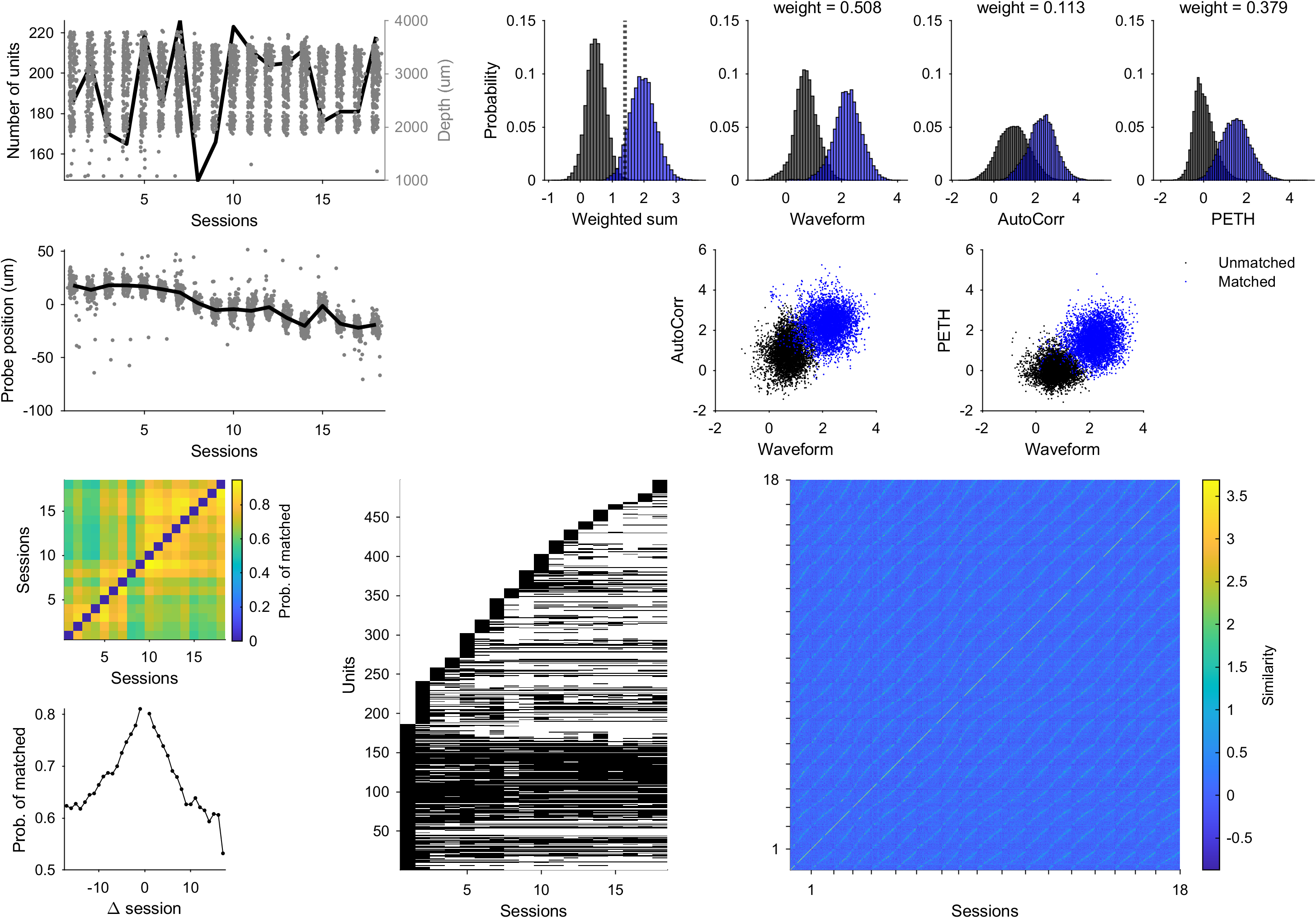
After running the code, you can inspect the results in Figures/Overview.png as shown above. You can also regenerate the figure in MATLAB by running:

overviewResults(user_settings, Output);

This figure summarizes the DANT results, including unit number and depth across sessions, estimated probe motion, similarity-score distributions for different features and their weights, matched probability between sessions, the presence of unique neurons across sessions, and the final similarity matrix. It gives you a quick way to assess tracking quality.

You may also want to inspect individual clusters more closely. Run the following code to visualize one cluster:

load DANT_Output/Output.mat; % load the output file
load DANT_Output/spikeInfo.mat; % load the spikeInfo file
load DANT_Output/Waveforms.mat; % load the waveforms file

cluster_id = 1; % specify the cluster ID you want to visualize

visualizeCluster(Output, cluster_id, spikeInfo, waveforms_corrected, Output.Params)

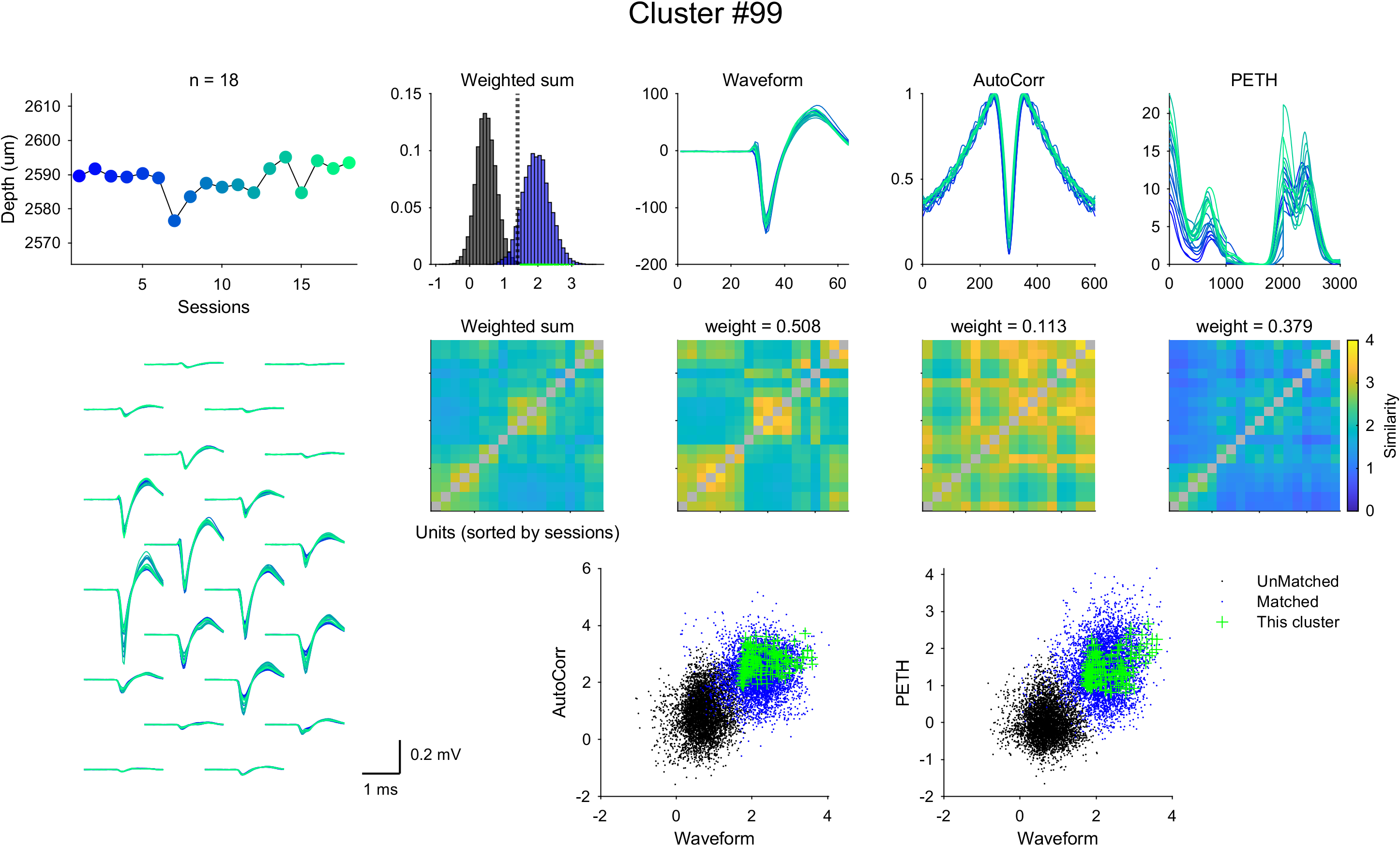
This generates a figure like the one above, showing the corrected depth, corrected waveforms, autocorrelograms, and PETHs of the units in the selected cluster, color-coded by session. It also shows the similarity between units within the cluster. The figure will be saved to Figures/Clusters/Cluster<cluster_id>.png.

Understand the output

Along with several intermediate files, the main output is stored in DANT_Output/Output.mat, which contains the following fields:

Field name	Type	Explanation
`RunTime`	1 x 1 double	total run time in seconds
`DateTime`	datetime string	date and time when the code is run
`NumUnits`	1 x 1 int	number of units included in the analysis
`NumSession`	1 x 1 int	number of sessions included in the analysis
`NumClusters`	1 x 1 int	number of clusters found (each cluster has at least 2 units)
`Sessions`	1 x n_unit int	session index for each unit
`Params`	1 x 1 struct	parameters used in the analysis (specified in `settings.json`)
`Locations`	n_unit x 3 double	estimated x, y, and z coordinates of each unit
`IdxCluster`	1 x n_unit int	cluster index for each unit
`ClusterMatrix`	n_unit x n_unit logical	cluster assignment matrix. `ClusterMatrix(i,j) = 1` means unit `i` and `j` are in the same cluster.
`MatchedPairs`	n_pairs x 2 int	unit index for all matched pairs
`IdxSort`	1 x n_unit int	sorted index of the units computed from hierarchical clustering algorithm (optimalleaforder)
`SimilarityNames`	1 x n_features cell	names of the similarity metrics used in the analysis
`SimilarityAll`	n_pairs x n_features double	similarity between each pair of units
`SimilarityPairs`	n_pairs x 2 int	unit index for each pair of units
`SimilarityWeights`	1 x n_features double	weights of the similarity metrics computed from IHDBSCAN algorithm
`SimilarityThreshold`	1 x 1 double	threshold used to determine the good matches in GoodMatchesMatrix
`GoodMatchesMatrix`	n_unit x n_unit logical	good matches determined by SimilarityThreshold
`SimilarityMatrix`	n_unit x n_unit double	weighted sum of the similarity between each pair of units
`Motion`	1 x 1 struct	estimated motion parameters across sessions
`CurationPairs`	n_pairs x 2 int	unit index for each pair of units that are curated
`CurationTypes`	1 x n_pairs int	types of curation for each pair of units
`CurationTypeNames`	1 x n_types cell	names of the curation types
`CurationNumRemoval`	1 x 1 int	number of pairs removed in the curation step

The most important field is IdxCluster, which assigns a unique cluster ID to each unit (-1 for non-matched units). You can use it to extract matched units across sessions. To learn more about the output, please refer to the Input and Output section.

Tracking is complete. You can now move on to cross-session analysis with the tracked neurons.